R Strip Chart

Step-by-Step Guide: Creating Strip Charts in R

Follow these detailed steps to create statistical strip charts in R using the stripchart() function

Prepare Data

Install the necessary R packages (Download R) for creating strip charts. The main packages you'll need are ggplot2, plotly, and dplyr for data manipulation.
Install R from r-project.org
Install RStudio (recommended IDE) Rstudio download now
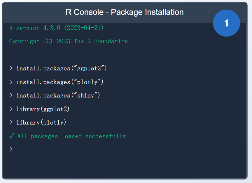
Run: install.packages(c("ggplot2", "plotly", "dplyr"))
Load packages: library(ggplot2)

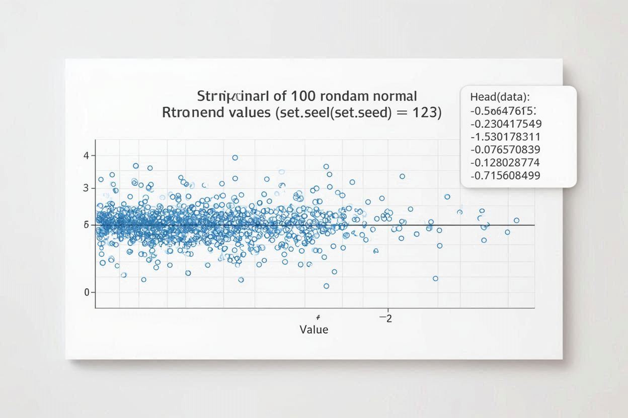
First, we need to prepare our data. Strip charts are ideal for displaying the distribution of small sample data. Let's create a numeric vector containing random numbers as sample data.

# Set random seed to ensure reproducible results
set.seed(123)

# Generate data with 100 random normally distributed values
data <- rnorm(100)

# View the first few data points
head(data)
# [1] -0.56047565 -0.23017749  1.55870831  0.07050839  0.12928774  1.71506499

Explanation: Using set.seed() ensures that the same data is generated each time you run the code, which is important for reproducibility. rnorm(100) generates 100 random numbers from a standard normal distribution.

Create Basic Strip Chart

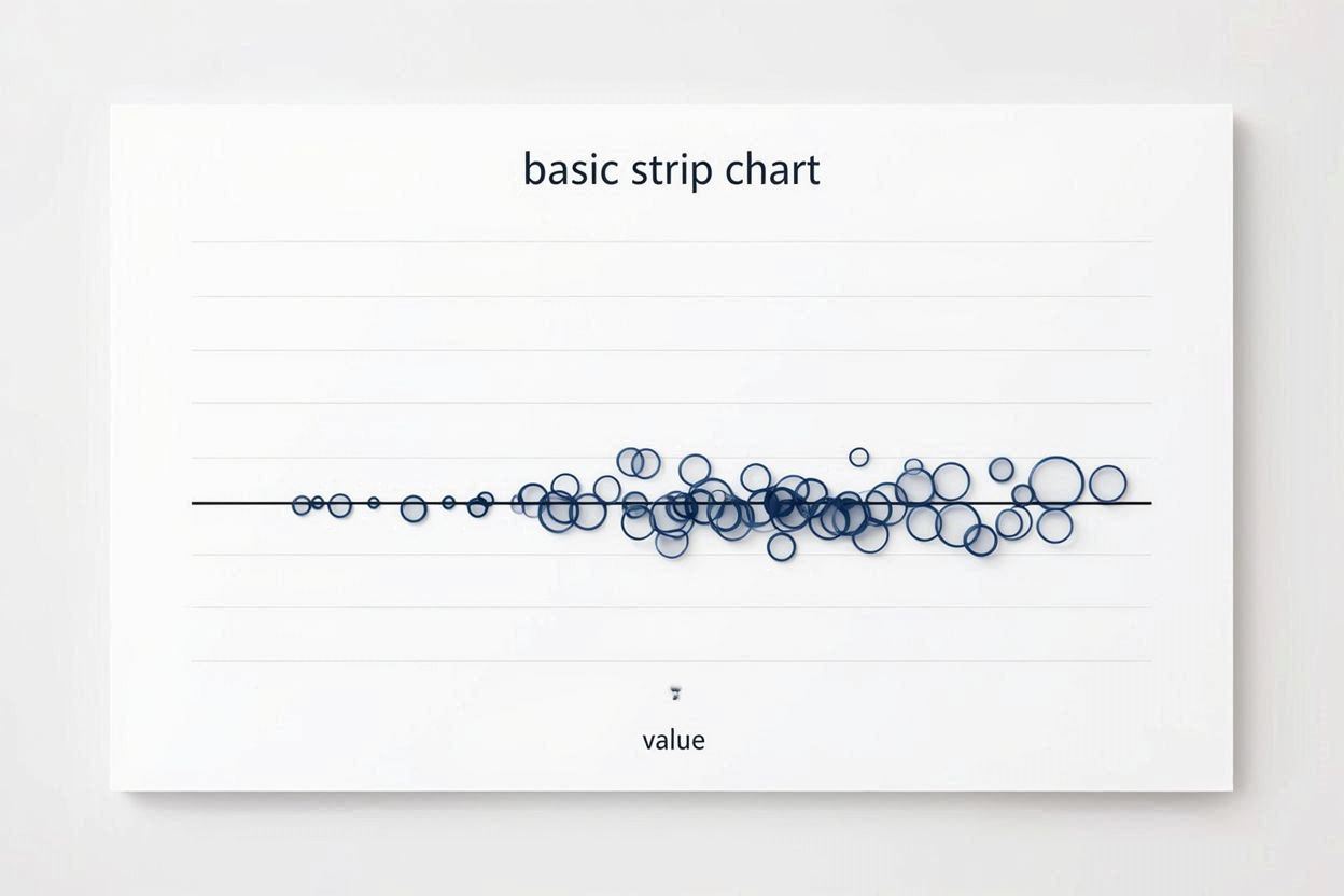
Use R's built-in stripchart() function to create a basic strip chart. This is the simplest one-dimensional scatter plot for displaying data distribution.

# Create basic strip chart
stripchart(data, 
           main = "Basic Strip Chart", 
           xlab = "Value")

# Result: Data points are arranged horizontally on a line, some points may overlap

Explanation: stripchart() is R's basic plotting function. By default, data points are arranged horizontally. If data points have duplicate values, they will overlap.

Customize Point Style

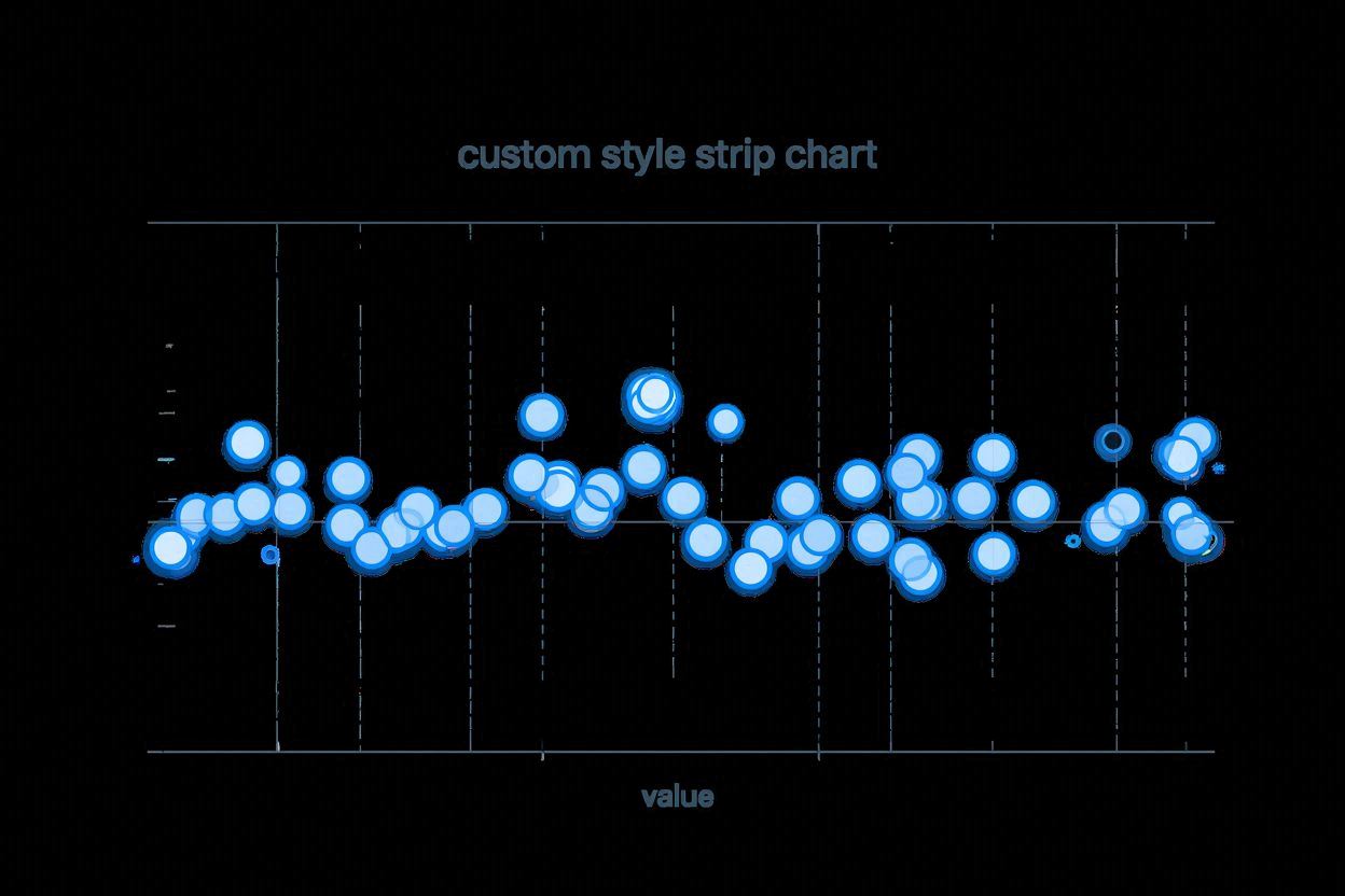
R Strip Chart Step 3 - Customized Points

Change the shape of points using the pch parameter and the color using the col parameter to make the chart more visually appealing.

# Customize point shape and color
stripchart(data, 
           pch = 21,           # Point shape (21 is filled circle)
           col = "blue",       # Border color
           bg = "lightblue",   # Fill color
           lwd = 2,            # Line width
           main = "Customized Strip Chart",
           xlab = "Value")

# Result: Data points displayed as circles with blue border and light blue fill

Explanation: The pch parameter controls point shape (1-25), col controls border color, and bg controls fill color (only effective when pch is 21-25).

Methods for Overlapping Points

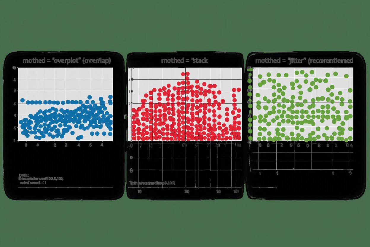
When data points have duplicate values, you can use three methods to handle overlaps: "overplot" (overlap), "stack" (stack), and "jitter" (jitter).

# Generate data with duplicate values
set.seed(1)
x <- round(runif(100, 0, 10))

# Method 1: Overplot (default method)
stripchart(x, 
           method = "overplot", 
           pch = 19, 
           col = "blue",
           main = "method = 'overplot'")

# Method 2: Stack
stripchart(x, 
           method = "stack", 
           pch = 19, 
           col = "red",
           main = "method = 'stack'")

# Method 3: Jitter (recommended)
stripchart(x, 
           method = "jitter", 
           pch = 19, 
           col = "green",
           jitter = 0.2,  # Jitter amount
           main = "method = 'jitter'")

Explanation:

"overplot": Duplicate points overlap directly, may be hard to see
"stack": Duplicate points are stacked vertically, similar to a histogram
"jitter": Adds random noise in the vertical direction to reduce overlap (most commonly used)

Vertical Strip Chart

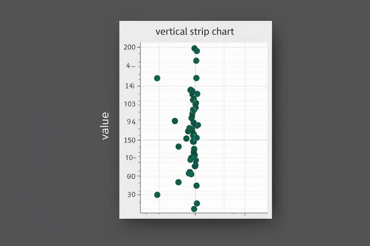
By setting the vertical = TRUE parameter, you can display the strip chart vertically, which may be more intuitive in certain situations.

# Create vertical strip chart
stripchart(data, 
           method = "jitter", 
           vertical = TRUE,    # Vertical display
           pch = 16, 
           col = "darkgreen",
           main = "Vertical Strip Chart",
           ylab = "Value")

# Result: Data points arranged vertically, Y-axis shows values

Explanation: When displayed vertically, values appear on the Y-axis, and the X-axis is typically used for grouping. This is particularly useful when comparing data distributions across multiple groups.

Group Comparison

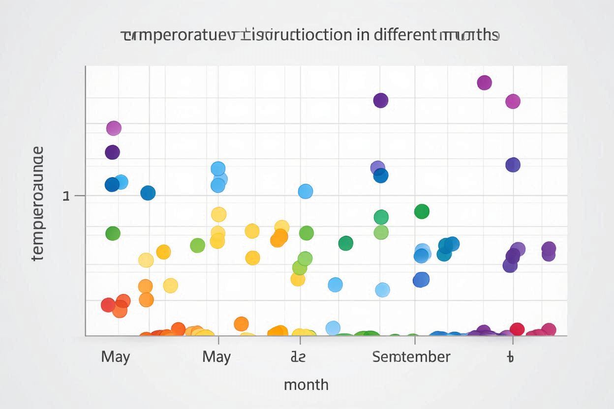
Use the formula syntax y ~ x to create strip charts by group, comparing data distributions across different groups.

# Use built-in airquality dataset to compare temperature by month
data("airquality")

# Create strip chart of temperature by month
stripchart(Temp ~ Month, 
           data = airquality, 
           method = "jitter", 
           vertical = TRUE,
           pch = 16, 
           col = rainbow(5),
           main = "Temperature Distribution by Month",
           xlab = "Month", 
           ylab = "Temperature")

# Or create custom grouped data
set.seed(1)
x <- rnorm(100)
groups <- sample(c("Group A", "Group B", "Group C"), 100, replace = TRUE)

stripchart(x ~ groups, 
           method = "jitter",
           jitter = 0.2,
           vertical = TRUE,
           pch = 19,
           col = c("red", "blue", "green"),
           main = "Group Comparison",
           xlab = "Group",
           ylab = "Value")

Explanation: In the formula syntax y ~ x, y is the numeric variable and x is the grouping variable (factor). This allows for intuitive comparison of data distribution differences across groups.

Add Statistical Information

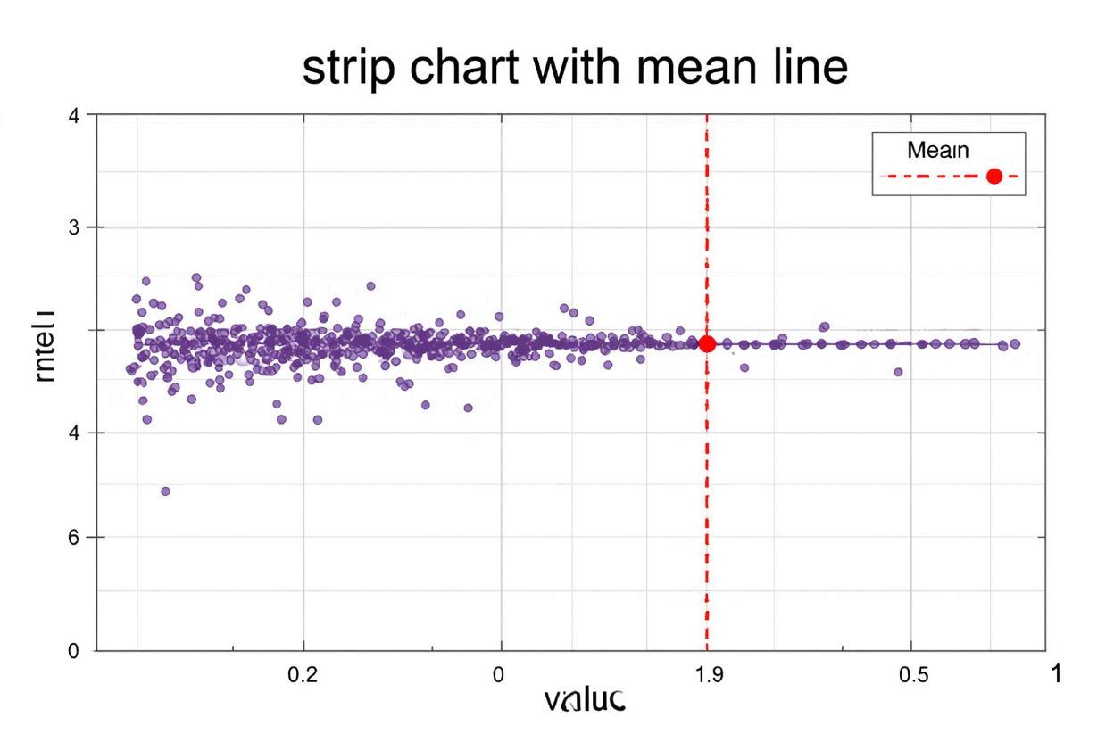
Adding mean lines or mean points to the strip chart can help better understand the central tendency of the data.

# Create strip chart
stripchart(data, 
           method = "jitter", 
           pch = 16, 
           col = "purple",
           main = "Strip Chart with Mean Line",
           xlab = "Value")

# Add mean line (use v= for horizontal charts)
abline(v = mean(data), 
       col = "red", 
       lwd = 2, 
       lty = 2)

# Add mean point
points(mean(data), 1, 
       pch = 19, 
       col = "red", 
       cex = 1.5)

# Add legend
legend("topright", 
       legend = c("Data Points", "Mean"), 
       pch = c(16, 19),
       col = c("purple", "red"),
       cex = 0.8)

# For vertical charts, use h= to add horizontal line
stripchart(data, 
           method = "jitter", 
           vertical = TRUE,
           pch = 16, 
           col = "blue",
           main = "Vertical Strip Chart with Mean Line",
           ylab = "Value")

abline(h = mean(data), 
       col = "red", 
       lwd = 2, 
       lty = 2)

Explanation: Use the abline() function to add reference lines. Use v= (vertical line) for horizontal charts and h= (horizontal line) for vertical charts. points() can add additional point markers.

Advanced Customization

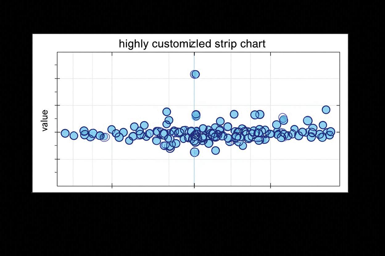
Further customize the chart appearance, including adjusting margins, adding grid lines, and other enhancements to make the chart more professional and visually appealing.

# Create highly customized strip chart
par(mar = c(5, 4, 4, 2) + 0.1)  # Set margins

stripchart(data, 
           method = "jitter",
           vertical = TRUE,
           pch = 21,
           col = "darkblue",
           bg = "lightblue",
           cex = 1.2,
           lwd = 1.5,
           frame.plot = TRUE,    # Show frame
           main = "Highly Customized Strip Chart",
           xlab = "",
           ylab = "Value",
           cex.main = 1.3,        # Title size
           cex.lab = 1.1,         # Axis label size
           cex.axis = 1.0)        # Axis tick size

# Add grid lines
grid(nx = NA, ny = NULL, col = "gray90", lty = "dotted")

# Add mean and median lines
abline(h = mean(data), col = "red", lwd = 2, lty = 2)
abline(h = median(data), col = "orange", lwd = 2, lty = 3)

# Add legend
legend("topright",
       legend = c("Data Points", "Mean", "Median"),
       pch = c(21, NA, NA),
       lty = c(NA, 2, 3),
       col = c("darkblue", "red", "orange"),
       bg = "white",
       cex = 0.9)

Explanation: Use the par() function to set graphical parameters, grid() to add grid lines, and legend() to add legends. These settings make the chart more professional and readable.

R Code Examples and Applications

Practical R code examples and real-world applications for statistical strip charts

Basic ggplot2 Strip Chart

# Load required libraries
library(ggplot2)
library(dplyr)

# Create sample time series data
set.seed(123)
time_series <- data.frame(
    time = seq(as.POSIXct("2024-01-01"), by = "1 min", length.out = 1000),
    value = cumsum(rnorm(1000, 0, 0.1))
)

# Create basic strip chart
strip_chart <- ggplot(time_series, aes(x = time, y = value)) +
    geom_line(color = "blue", size = 1) +
    labs(
        title = "Real-time Strip Chart",
        x = "Time",
        y = "Value"
    ) +
    theme_minimal() +
    theme(
        plot.title = element_text(hjust = 0.5),
        axis.text.x = element_text(angle = 45, hjust = 1)
    )

# Display the chart
print(strip_chart)

Explanation:

This basic implementation creates a simple strip chart using ggplot2. The code generates sample time series data and creates a clean, professional-looking line chart with proper formatting.

Multi-Channel Strip Chart with Statistical Analysis

# Multi-channel strip chart with statistical analysis
library(ggplot2)
library(dplyr)
library(tidyr)

# Generate multi-channel data
set.seed(123)
multi_data <- data.frame(
    time = seq(as.POSIXct("2024-01-01"), by = "1 min", length.out = 1000),
    temperature = 20 + cumsum(rnorm(1000, 0, 0.1)),
    pressure = 50 + cumsum(rnorm(1000, 0, 0.2)),
    flow_rate = 10 + cumsum(rnorm(1000, 0, 0.15))
)

# Reshape data for plotting
multi_data_long <- multi_data %>%
    pivot_longer(cols = c(temperature, pressure, flow_rate),
                 names_to = "variable", values_to = "value")

# Create multi-channel strip chart
multi_strip_chart <- ggplot(multi_data_long, aes(x = time, y = value, color = variable)) +
    geom_line(size = 1) +
    geom_smooth(method = "loess", se = TRUE, alpha = 0.3) +
    labs(
        title = "Multi-Channel Strip Chart with Trend Analysis",
        x = "Time",
        y = "Value",
        color = "Variable"
    ) +
    scale_color_manual(values = c("temperature" = "red", 
                                 "pressure" = "blue", 
                                 "flow_rate" = "green")) +
    theme_minimal() +
    theme(
        plot.title = element_text(hjust = 0.5),
        legend.position = "bottom"
    )

print(multi_strip_chart)

Explanation:

This example shows how to create a multi-channel strip chart with statistical trend analysis. It demonstrates data reshaping, multiple variables, and trend line fitting using LOESS smoothing.

Interactive Strip Chart with plotly

# Interactive strip chart with plotly
library(ggplot2)
library(plotly)
library(dplyr)

# Create advanced strip chart
create_interactive_strip_chart <- function(data, title = "Interactive Strip Chart") {
    # Create ggplot2 base
    p <- ggplot(data, aes(x = time, y = value)) +
        geom_line(color = "blue", size = 1) +
        geom_smooth(method = "loess", se = TRUE, alpha = 0.3, color = "red") +
        labs(
            title = title,
            x = "Time",
            y = "Value"
        ) +
        theme_minimal() +
        theme(plot.title = element_text(hjust = 0.5))
    
    # Convert to plotly
    plotly_chart <- ggplotly(p, tooltip = c("x", "y")) %>%
        layout(
            title = list(text = title),
            xaxis = list(title = "Time"),
            yaxis = list(title = "Value"),
            hovermode = "x unified"
        ) %>%
        config(displayModeBar = TRUE)
    
    return(plotly_chart)
}

# Generate sample data
set.seed(123)
sample_data <- data.frame(
    time = seq(as.POSIXct("2024-01-01"), by = "1 min", length.out = 500),
    value = cumsum(rnorm(500, 0, 0.1)) + sin(seq(0, 4*pi, length.out = 500))
)

# Create interactive chart
interactive_chart <- create_interactive_strip_chart(sample_data, "Real-time Data Analysis")
print(interactive_chart)

Explanation:

This advanced implementation creates an interactive strip chart using plotly. It includes trend analysis, hover information, and web-ready interactivity for enhanced user experience.

R Introduction

What is R?

Key Features

Main Applications

Advantages of Using R for Strip Charts

Free and Open Source

Statistical Excellence

Rich Package Ecosystem

Reproducible Research

Strong Community

High Customization

Step-by-Step Guide: Creating Strip Charts in R

Prepare Data

Create Basic Strip Chart

Customize Point Style

Methods for Overlapping Points

Vertical Strip Chart

Group Comparison

Add Statistical Information

Advanced Customization

R Code Examples and Applications

Basic ggplot2 Strip Chart

Explanation:

Multi-Channel Strip Chart with Statistical Analysis

Explanation:

Interactive Strip Chart with plotly

Explanation:

R Strip Chart Applications

Scientific Research and Analysis

Quality Control and Statistical Process Control

Academic Research and Education